How to Calculate an Interval Estimate
— Step-by-Step Guide
One number alone rarely tells the full story. This guide walks you through every method, formula, and worked example you need to calculate confident, accurate interval estimates — from confidence intervals for means to proportions, Z-scores to T-distributions.
What Is an Interval Estimate?
Imagine you surveyed 200 Americans about their monthly grocery spending and found an average of $520. If you report that number alone — “the average American spends $520/month on groceries” — you’re making a point estimate. It sounds precise, but it hides a critical question: how precise is it really?
An interval estimate solves this by giving you a range instead of a single value: “We are 95% confident the true average falls between $497 and $543.” That range communicates both your best guess and the natural uncertainty in your sample data.
The Core Idea An interval estimate = Point Estimate ± Margin of Error. The margin of error reflects sample size, data variability, and how confident you want to be. Larger samples → smaller margins → tighter, more precise intervals.
In statistics, the most common type of interval estimate is the confidence interval (CI). You’ve seen them everywhere — in election polls (“Candidate A leads 52% to 44%, margin of error ±3%”), medical studies, economic reports, and product quality testing. They are the foundation of honest, transparent data communication.
By the Numbers Research published in PLOS Medicine found that a significant portion of published clinical trial reports omit confidence intervals entirely — forcing readers to rely on p-values alone, which tell you far less about the practical significance of results. The American Statistical Association specifically recommends interval estimates as a key tool for more transparent science.

Key Terms You Must Understand First
Before you touch a formula, make sure these terms are locked in. They come up in every calculation.
| Term | Symbol | What It Means | Example |
|---|---|---|---|
| Population | N | The entire group you want to draw conclusions about | All registered voters in the US |
| Sample | n | The smaller group you actually measured | 1,200 randomly selected voters |
| Sample Mean | x̄ | The average of your sample data — your point estimate for the population mean | x̄ = $520 average spend |
| Population Mean | μ | The true average of the entire population (usually unknown — what we’re estimating) | μ = ? (what we’re finding) |
| Standard Deviation | σ or s | How spread out individual data values are. σ = population (known), s = sample (calculated) | s = $85 spread in spending |
| Standard Error (SE) | SE | How much the sample mean varies across different samples. SE = s / √n | SE = $85 / √200 = $6.01 |
| Confidence Level | CL | How often your method will capture the true value in repeated sampling (90%, 95%, 99%) | 95% confidence level |
| Critical Value | z* or t* | The multiplier from the Z or T distribution that matches your confidence level | z* = 1.96 for 95% CI |
| Margin of Error | ME | The amount added/subtracted from the point estimate. ME = critical value × SE | ME = 1.96 × $6.01 = $11.78 |
| Degrees of Freedom | df | Used in T-distributions. df = n − 1 for a single sample mean | n=25 → df=24 |
| Significance Level | α | The probability of your interval missing the true value. α = 1 − confidence level | 95% CI → α = 0.05 |
Confidence Level vs. Confidence Interval — Don’t Mix These Up The confidence level (e.g., 95%) describes the method’s reliability across many samples. The confidence interval (e.g., $497 to $543) is the specific range produced by one sample. A 95% confidence level means: if you repeated your study 100 times, about 95 of those 100 intervals would contain the true population value.

Types of Interval Estimates
| Type | What It Estimates | Width | Best Used For | USA Example |
|---|---|---|---|---|
| Confidence Interval (CI) | Where the population mean or proportion likely falls | Moderate | Research, surveys, quality control | Election poll: “52% ± 3%” support for a candidate |
| Prediction Interval (PI) | Where a single future observation likely falls | Wider than CI | Forecasting, individual-level decisions | Predicting the delivery time of a single FedEx package |
| Tolerance Interval (TI) | Range covering a set proportion of the population | Widest | Engineering, manufacturing, compliance | FDA: “90% of patients will have blood pressure in this range” |
For most students, researchers, and analysts, confidence intervals are the focus. This guide covers CIs in depth — specifically for population means and population proportions, which cover the vast majority of real-world needs.
Why Prediction Intervals Are Always Wider A confidence interval captures uncertainty about the average. A prediction interval must also account for the natural variation of individual observations around that average — so it’s always wider. If a CI for mean package delivery is 2.1 to 2.4 days, the PI for a single package might be 1.0 to 3.5 days.
The Core Formula — Broken Down Symbol by Symbol
Formula A — Confidence Interval for a Population Mean
CI for Mean — Population Standard Deviation Known (Z-interval)
CI = x̄±z* × (σ/ √n)
x̄Sample mean — your best single estimate
z*Critical Z-value for your chosen confidence level
σPopulation standard deviation (must be known)
nSample size — number of observations
σ/√nStandard error of the mean (SE)
±Creates the lower and upper bounds of the interval
Formula B — Confidence Interval for a Population Mean (σ unknown)
CI for Mean — Population Standard Deviation Unknown (T-interval) — Most Common in Practice
CI = x̄±t* × (s/ √n)
x̄Sample mean
t*Critical T-value with df = n − 1 degrees of freedom
sSample standard deviation (calculated from your data)
nSample size
s/√nEstimated standard error of the mean
dfn − 1 (used to look up t* in T-table)
Formula C — Confidence Interval for a Population Proportion
CI for Proportion (used in polls, surveys, quality testing)
CI = p̂±z* × √(p̂(1−p̂) /n)
p̂Sample proportion (e.g., 0.52 = 52% said yes)
z*Critical Z-value (proportion CIs always use Z, not T)
1−p̂Complement of the sample proportion
nSample size
√(p̂(1−p̂)/n)Standard error of the proportion
Use Condition for Proportion CI Before using Formula C, verify: n × p̂ ≥ 10 AND n × (1 − p̂) ≥ 10. If this condition fails (very small samples or extreme proportions near 0 or 1), use Wilson Score Interval or an exact method instead.
Z-Score vs. T-Score | The Definitive Decision Guide
This is where many students get tripped up. The wrong choice inflates or deflates your interval. Here’s the clear framework:
| Use Z-Score (Z-Critical) When | Use T-Score (T-Critical) When |
|---|---|
| Sample size is large (n ≥ 30) | Sample size is small (n < 30) |
| Population standard deviation (σ) is known | Population standard deviation (σ) is unknown |
| Estimating a proportion (p̂) | Estimating a mean with limited data |
| Data is approximately normally distributed | Data is roughly bell-shaped |
| Common in national surveys, polls, and quality control | Common in lab studies, pilot research, and small clinical trials |
The “Gray Zone” (n = 30–50) When n is between 30 and 50 and σ is unknown, both methods give similar results. Most statisticians default to the T-distribution in this range because it’s more conservative (slightly wider intervals), which is safer. As n → ∞, the T-distribution converges to the Z-distribution anyway.

Critical Value Tables (Z and T) — Bookmark Reference
Z Critical Values (most commonly used)
| Confidence Level | α (Significance Level) | α/2 (Two-Tailed) | Z Critical Value (z*) | Common Use |
|---|---|---|---|---|
| 80% | 0.20 | 0.10 | 1.282 | Rough estimates, low-stakes decisions |
| 85% | 0.15 | 0.075 | 1.440 | Exploratory studies |
| 90% | 0.10 | 0.050 | 1.645 | Social science research, business reports |
| 95% | 0.05 | 0.025 | 1.960 | ⭐ Most common standard in research & polling |
| 98% | 0.02 | 0.010 | 2.326 | Stricter scientific publications |
| 99% | 0.01 | 0.005 | 2.576 | Medical studies, safety-critical applications |
| 99.9% | 0.001 | 0.0005 | 3.291 | Pharmaceutical approvals, nuclear safety |
T Critical Values by Degrees of Freedom (df = n − 1)
| df (n−1) | Sample Size n | t* for 90% CI | t* for 95% CI | t* for 99% CI |
|---|---|---|---|---|
| 4 | 5 | 2.132 | 2.776 | 4.604 |
| 9 | 10 | 1.833 | 2.262 | 3.250 |
| 14 | 15 | 1.761 | 2.145 | 2.977 |
| 19 | 20 | 1.729 | 2.093 | 2.861 |
| 24 | 25 | 1.711 | 2.064 | 2.797 |
| 29 | 30 | 1.699 | 2.045 | 2.756 |
| 49 | 50 | 1.677 | 2.010 | 2.682 |
| 99 | 100 | 1.660 | 1.984 | 2.626 |
| ∞ | Large | 1.645 | 1.960 | 2.576 |
As df increases (larger samples), T critical values shrink toward Z critical values. With df = ∞ (infinite sample), T and Z are identical. This is why large-sample T intervals and Z intervals give essentially the same answer.
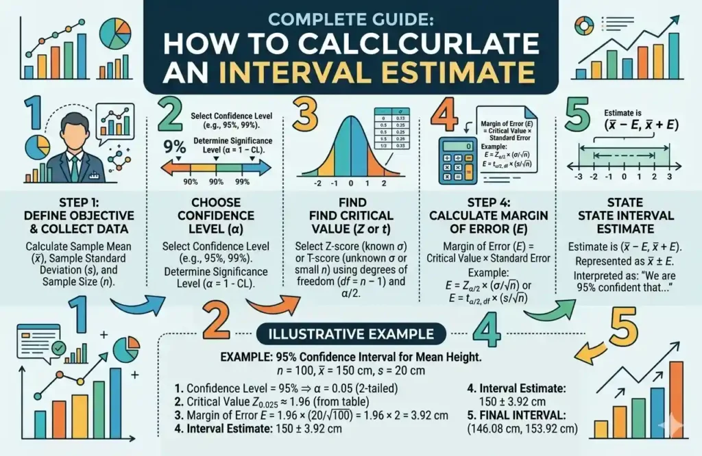
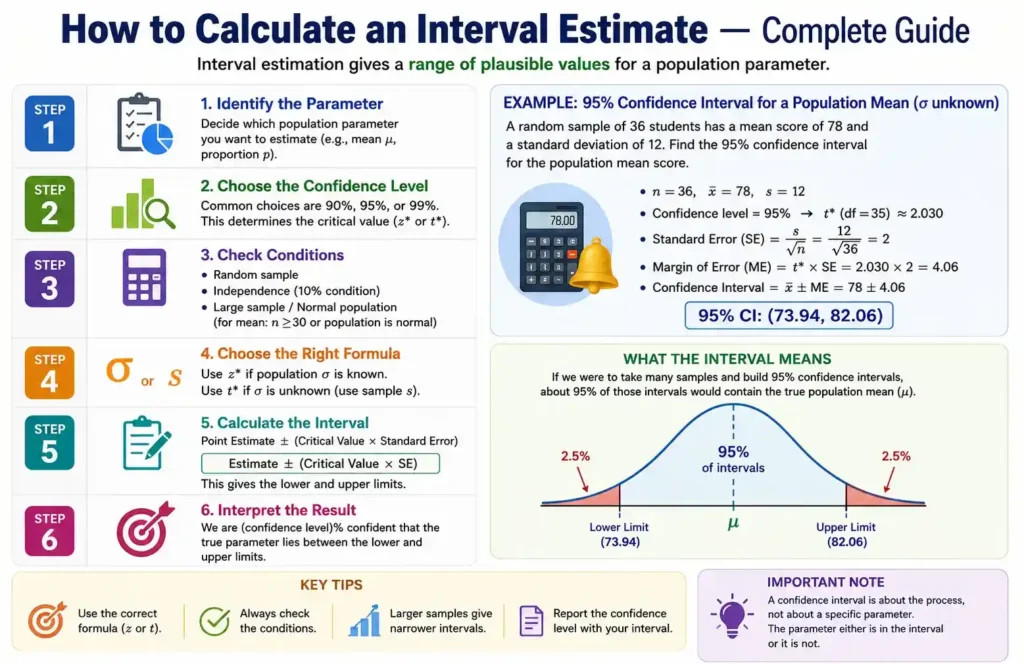
Step Process to Calculate Any Interval Estimate
Follow these six steps for any interval estimate calculation — regardless of whether you’re working with means, proportions, Z, or T.
Identify What You’re Estimating
Are you estimating a population mean (μ) or a population proportion (p)? This determines which formula to use. Mean → use Formula A or B. Proportion → use Formula C.
Collect and Summarize Your Sample Data
Record your sample size n, sample mean x̄ (or proportion p̂), and standard deviation s (or σ if population SD is known). Verify your sample was randomly drawn — biased samples make any CI meaningless.
Choose Your Confidence Level
Decide: 90%, 95%, or 99%. Use 95% as your default unless your field or context requires otherwise. Higher confidence = wider interval = less precise, but more reliable.
Determine Z* or T* (Critical Value)
Use Z* if n ≥ 30 and σ is known, or if estimating a proportion. Use T* (with df = n − 1) if n < 30 or σ is unknown. Look up the value in the tables above.
Calculate the Margin of Error (ME)
For means: ME = z* × (σ/√n) or ME = t* × (s/√n)
For proportions: ME = z* × √(p̂(1−p̂)/n)
This is the ± amount in your final interval.
Build & Interpret the Interval
Lower bound = Point Estimate − ME · Upper bound = Point Estimate + ME
State it clearly: “We are [confidence level]% confident the true [parameter] falls between [lower] and [upper].” Always interpret in context — never just report numbers.
Average American Credit Card Debt — Large Sample, σ Known
A financial researcher samples n = 400 American households to estimate average credit card debt. Population σ = $1,200. Sample mean x̄ = $6,800. Desired confidence: 95%.
Identify: Estimating a population mean. σ is known. n = 400 ≥ 30 → Use Z-interval (Formula A).
Summarize data: x̄ = $6,800, σ = $1,200, n = 400
Confidence level = 95% → Z-critical value z* = 1.960
Standard Error: SE = σ/√n = $1,200 / √400 = $1,200 / 20 = $60
Margin of Error: ME = 1.960 × $60 = $117.60
Interval: $6,800 ± $117.60 → ($6,682.40, $6,917.60)
We are 95% confident the true average credit card debt of all American households falls between $6,682.40 and $6,917.60.
Example 2 · CI for Mean · Small Sample · T-interval
Average Hospital Stay Duration — Small Clinical Sample, σ Unknown
Scenario: A hospital administrator reviews n = 16 recent patient records. Sample mean length of stay x̄ = 4.5 days. Sample standard deviation s = 1.2 days. σ unknown. Desired confidence: 95%.
n = 16 < 30, σ unknown → Use T-interval (Formula B). df = n − 1 = 15.
Data: x̄ = 4.5 days, s = 1.2 days, n = 16
95% CI with df = 15 → T-critical value: t* = 2.131 (from T-table)
Standard Error: SE = s/√n = 1.2 / √16 = 1.2 / 4 = 0.30 days
Margin of Error: ME = 2.131 × 0.30 = 0.639 days
Interval: 4.5 ± 0.639 → (3.86 days, 5.14 days)
We are 95% confident the true mean hospital stay for this patient population falls between 3.86 and 5.14 days.
Example 3 · CI for Proportion · Election Polling
Presidential Approval Rating — National Poll
Scenario: A polling firm surveys n = 1,200 registered American voters. 648 say “approve”. Calculate a 95% confidence interval for the true approval proportion.
Estimating a proportion → Use Formula C. Check conditions: n×p̂ = 1200×0.54 = 648 ≥ 10 ✓. n×(1−p̂) = 1200×0.46 = 552 ≥ 10 ✓
Sample proportion: p̂ = 648 / 1,200 = 0.54 (54%)
95% CI → Z-critical: z* = 1.960
Standard Error: SE = √(0.54 × 0.46 / 1,200) = √(0.2484/1200) = √0.000207 = 0.01439
Margin of Error: ME = 1.960 × 0.01439 = 0.02820 ≈ ±2.8%
Interval: 0.54 ± 0.028 → (51.2%, 56.8%)
Conclusion: We are 95% confident the true approval rating among all registered voters is between 51.2% and 56.8%. The margin of error is ±2.8%.
Example 4 · CI for Mean · Comparing Confidence Levels
How Confidence Level Width Changes — SAT Score Study
Scenario: SAT coaching program samples n = 64 students. x̄ = 1,180 points. s = 96 points. Calculate intervals at 90%, 95%, and 99% to see how width changes.
SE = s/√n = 96/√64 = 96/8 = 12 points. Since n = 64 ≥ 30, use Z-scores.
| Confidence Level | z* | ME = z* × SE | Lower Bound | Upper Bound | Interval Width |
|---|---|---|---|---|---|
| 90% | 1.645 | 1.645 × 12 = 19.7 | 1,160.3 | 1,199.7 | 39.4 pts |
| 95% | 1.960 | 1.960 × 12 = 23.5 | 1,156.5 | 1,203.5 | 47.0 pts ⭐ |
| 99% | 2.576 | 2.576 × 12 = 30.9 | 1,149.1 | 1,210.9 | 61.8 pts |
Key insight: Higher confidence = wider interval. To be 99% sure (vs. 95%), the interval grows by 14.8 points in each direction. There is always a precision-vs-certainty tradeoff.
Example 5 · CI for Proportion · Quality Control
Product Defect Rate — Manufacturing Quality Audit
Scenario: A QA manager at a US electronics factory inspects a batch of n = 500 units. 18 are defective. Construct a 99% CI for the true defect rate.
p̂ = 18/500 = 0.036 (3.6%). Check: n×p̂ = 18 ≥ 10 ✓, n×(1−p̂) = 482 ≥ 10 ✓
99% CI → z* = 2.576
SE = √(0.036 × 0.964 / 500) = √(0.034704/500) = √0.0000694 = 0.00833
ME = 2.576 × 0.00833 = 0.02146 ≈ 2.1%
Interval: 3.6% ± 2.1% → (1.5%, 5.7%)
We are 99% confident the true defect rate for this production line falls between 1.5% and 5.7%. The company can use this to set quality thresholds and schedule maintenance.
Real-World USA Applications of Interval Estimates
Interval estimates aren’t just textbook exercises. They’re embedded in nearly every data-driven field across the United States.
Election Polling
The “±3%” you see in every Gallup, Quinnipiac, and AP/VoteCast poll is a margin of error from a 95% CI for a proportion. It quantifies sampling uncertainty for millions of voters.
Clinical Medicine
FDA drug approvals and NIH-funded trials require confidence intervals on treatment effect sizes. A drug that lowers blood pressure by “8–14 mmHg (95% CI)” is interpreted very differently from one showing “11 mmHg” alone.
Finance & Economics
Federal Reserve economic forecasts, Bureau of Labor Statistics job reports, and Wall Street earnings models all use interval estimates to communicate uncertainty in projections like GDP growth and unemployment.
Manufacturing QC
Six Sigma and ISO 9001 quality systems use tolerance intervals to certify that production meets spec — e.g., “99% of parts will have a diameter between 9.97mm and 10.03mm.”
Education Research
NAEP (National Assessment of Educational Progress) reports state-level reading and math scores with explicit confidence intervals to reflect sampling uncertainty across diverse school populations.
Climate Science
NOAA temperature anomaly reports and IPCC projections present intervals like “global average temperature rise of 1.5°C–4.5°C” to communicate the honest range of model uncertainty.
A/B Testing
Amazon, Google, and Shopify run thousands of A/B tests where CI for conversion rate differences determines whether a new feature “significantly” outperforms the old one.
Legal & Forensics
Statistical evidence in discrimination cases, epidemiological studies in tort litigation, and forensic DNA match statistics all rely on interval-based uncertainty reporting in US federal courts.
Mistakes That Ruin Your Interval Estimate
- Misinterpreting the confidence level A 95% CI does NOT mean “there is a 95% probability the true value is in this interval.” The true parameter is fixed — it’s either in there or it isn’t. The 95% refers to the method’s long-run reliability across repeated samples. This is one of the most widespread misconceptions in statistics education.
- Using Z when you should use T (or vice versa) Small sample (n < 30) with unknown σ and you used z* = 1.96? Your interval is too narrow and overconfident. Always check sample size and whether σ is known before choosing your critical value.
- Ignoring the randomness assumption Confidence intervals are only valid when data comes from a random (or at least representative) sample. A convenience sample — like only surveying your Facebook friends — produces a CI that may be mathematically correct but practically meaningless.
- Failing to check the normality condition CI formulas assume the sampling distribution of the mean is approximately normal. For means, the Central Limit Theorem protects you when n ≥ 30. For very small samples (< 15) with heavily skewed data, standard CI formulas break down — consider bootstrap intervals.
- Forgetting to check the proportion condition For proportion CIs, you must verify n×p̂ ≥ 10 AND n×(1−p̂) ≥ 10. Surveys with very extreme proportions (e.g., a rare disease with p̂ = 0.002) violate this — use exact methods or Wilson Score intervals instead.
- Reporting the interval without interpretation Writing “(47.3, 52.7)” without context is incomplete. Always state: the confidence level, what parameter is being estimated, and what the interval means for your real-world question. Numbers without interpretation are data, not insight.
- Thinking a wider CI is always “worse”A wide CI isn’t a failure — it’s honest. If your data has high variability or a small sample, a wide interval is the truthful result. The mistake is artificially narrowing it by unjustifiably using a lower confidence level just to look more precise.
Best Tools & Calculators for Computing Interval Estimates in 2025
You don’t always need to calculate by hand. These tools are widely used by US students, researchers, and analysts:
Python (scipy.stats)
The gold standard for data science. stats.t.interval() and proportion_confint() in statsmodels handle every scenario.
R Language
t.test() and prop.test() return CIs automatically. Standard in academic research and biostatistics across the US.
Excel / Google Sheets
CONFIDENCE.NORM() for Z-intervals and CONFIDENCE.T() for T-intervals. Great for business analysts without coding backgrounds.
GraphPad Prism
Widely used in US biomedical and clinical research. Outputs CIs for nearly every statistical test with publication-ready graphs.
StatCrunch / SPSS
Classroom tools used extensively in US universities. Point-and-click CI calculation without coding required.
Confidence Interval Calculators (Online)
Sites like StatDistributions.com, Zeal Analytics, and Social Science Statistics offer free web-based CI calculators — no software needed.
Quick Python Code for a 95% T-Intervalimport scipy.stats as stats
import numpy as np
data = [4.2, 5.1, 3.8, 4.9, 5.3, 4.6, 3.7, 5.0] # your sample
ci = stats.t.interval(0.95, df=len(data)-1,
loc=np.mean(data), scale=stats.sem(data))
print(f"95% CI: {ci[0]:.3f} to {ci[1]:.3f}")
Frequently Asked Questions
What is the difference between a confidence interval and a margin of error?
The margin of error (ME) is the ± amount that defines how far the interval extends above and below the point estimate. The confidence interval is the complete range you get by applying that margin: lower bound = point estimate − ME, upper bound = point estimate + ME. When news outlets report “margin of error ±3%,” that single number implicitly defines a confidence interval. They are two sides of the same coin.
How does sample size affect the interval estimate?
Larger samples produce narrower, more precise intervals — because the standard error (SE = σ/√n or s/√n) shrinks as n grows. Doubling your sample size cuts the standard error by about 29% (by a factor of √2). This is why national polls use 1,000–1,500 respondents — below about 400–500, the margins become too wide to be meaningful for most decisions.
Can I construct a one-sided (one-tailed) confidence interval?
Yes. A one-sided CI is used when you only care about one direction — e.g., “the mean is at least X” or “the defect rate is at most Y.” For a one-sided 95% CI, use z* = 1.645 (not 1.960), because you’re putting all the 5% α in one tail. One-sided CIs are common in safety testing, drug efficacy (minimum effective dose), and engineering reliability.
What if my data is not normally distributed?
For large samples (n ≥ 30), the Central Limit Theorem means the sampling distribution of the mean is approximately normal regardless of the original data distribution — your standard CI formulas still work well. For small samples with skewed data, consider: (1) transforming the data (log transform), (2) using a bootstrap confidence interval, which makes no normality assumptions, or (3) using a non-parametric test. Bootstrap CIs are increasingly standard in modern data science.
What sample size do I need to achieve a specific margin of error?
For a desired ME, rearrange the formula: n = (z* × σ / ME)² for means, or n = (z*)² × p̂(1−p̂) / ME² for proportions. Example: for a 95% CI on a proportion with ME = ±3% (0.03) using p̂ = 0.5 (most conservative): n = (1.96)² × 0.25 / (0.03)² = 3.8416 × 0.25 / 0.0009 = 1,067. This is why most national polls use ~1,000–1,100 respondents for ±3% precision.
How is a confidence interval different from a Bayesian credible interval?
This is a deep and important distinction. A frequentist CI (what this guide covers) says: “If I repeated this study many times, 95% of computed intervals would contain the true parameter.” A Bayesian credible interval says: “Given my prior beliefs and this data, there is a 95% probability the true parameter falls in this range.” The Bayesian version is closer to what most people intuitively want, but requires specifying a prior distribution. Bayesian credible intervals are increasingly used in modern data science, A/B testing, and Bayesian clinical trials.
Why does a 99% confidence interval not mean I’m “more right” than with a 95% CI?
Both intervals are computed correctly from the same data — neither is “more right.” The 99% CI is simply wider, which means it captures more possible values and therefore has a higher chance of including the true parameter. You’re trading precision (a narrower, more informative range) for certainty (a higher probability of not missing the truth). Which tradeoff is appropriate depends on the stakes: safety-critical decisions warrant 99%, while exploratory research often accepts 90%.
Ready to Apply Interval Estimates in Your Work?
Whether you’re analyzing survey data, running A/B tests, or reporting research findings — mastering interval estimates puts you in a small group of professionals who communicate uncertainty honestly and persuasively
This guide covers frequentist confidence interval construction following standard methods from introductory and applied statistics. Formulas verified against Moore, McCabe & Craig Introduction to the Practice of Statistics and Montgomery & Runger Applied Statistics and Probability for Engineers.